Supervised Learning I: classification
Overview
Teaching: 20 min
Exercises: 10 minQuestions
How can I apply supervised learning to a data set?
Objectives
Know the basic Machine Learning terminology.
Build a model to predict a categorical target variable.
Apply logistic regression and random forests algorithms to a data set and compare them.
Learn the importance of separating data into training and test sets.
Supervised Learning I: classification
As mentioned in passing before: Supervised learning, is the branch of machine learning that involves predicting labels, such as whether a tumour will be benign or malignant.
In this section, you’ll attempt to predict tumour diagnosis based on geometrical measurements.
Discussion
Look at your pair plot. What would a baseline model there be?
Exercise
Build a model that predicts diagnosis based on whether
X3 > 15or something similar.Solution
# Build baseline model
df$pred <- ifelse(df$X3 > 15, "M", "B")
df$pred
This is not a great model but it does give us a baseline: any model that we build later needs to perform better than this one.
Whoa: what do we mean by model performance here? There are many metrics to determine model performance and here we’ll use accuracy, the percentage of the data that the model got correct.
Note on terminology
- The target variable is the one you are trying to predict;
- Other variables are known as features (or predictor variables).
We first need to change df$X2, the target variable, to a factor:
# What is the class of X2?
class(df$X2)
[1] "character"
# Change it to a factor
df$X2 <- as.factor(df$X2)
# What is the class of X2 now?
class(df$X2)
[1] "factor"
Calculate baseline model accuracy:
# Calculate accuracy
confusionMatrix(as.factor(df$pred), df$X2)
Confusion Matrix and Statistics

          Reference
Prediction   B   M
         B 345  51
         M  12 161

               Accuracy : 0.8893
                 95% CI : (0.8606, 0.9139)
    No Information Rate : 0.6274
    P-Value [Acc > NIR] : < 2.2e-16

                  Kappa : 0.754
 Mcnemar's Test P-Value : 1.688e-06

            Sensitivity : 0.9664
            Specificity : 0.7594
         Pos Pred Value : 0.8712
         Neg Pred Value : 0.9306
             Prevalence : 0.6274
         Detection Rate : 0.6063
   Detection Prevalence : 0.6960
      Balanced Accuracy : 0.8629

       'Positive' Class : B
Now it’s time to build an ever so slightly more complex model, a logistic regression.
Logistic regression
Let’s build a logistic regression. You can read more about how logistic works here and the instructor may show you some motivating and/or explanatory equations on the white/chalk-board. What’s important to know is that logistic regression is used for classification problems (such as our case of predicting whether a tumour is benign or malignant).
Note on logistic regression
Logistic regression, or logreg, outputs a probability, which you’ll then convert to a prediction.
Now build that logreg model:
# Build model
model <- glm(X2 ~ ., family = "binomial", df)
Warning: glm.fit: algorithm did not converge
Warning: glm.fit: fitted probabilities numerically 0 or 1 occurred
# Predict probability on the same dataset
p <- predict(model, df, type="response")
# Convert probability to prediction "M" or "B"
pred <- ifelse(p > 0.50, "M", "B")

# Create confusion matrix
confusionMatrix(as.factor(pred), df$X2)
Confusion Matrix and Statistics

          Reference
Prediction   B   M
         B 357   0
         M   0 212

               Accuracy : 1
                 95% CI : (0.9935, 1)
    No Information Rate : 0.6274
    P-Value [Acc > NIR] : < 2.2e-16

                  Kappa : 1
 Mcnemar's Test P-Value : NA

            Sensitivity : 1.0000
            Specificity : 1.0000
         Pos Pred Value : 1.0000
         Neg Pred Value : 1.0000
             Prevalence : 0.6274
         Detection Rate : 0.6274
   Detection Prevalence : 0.6274
      Balanced Accuracy : 1.0000

       'Positive' Class : B
Discussion
From the above, can you say what the model accuracy is?
Also, don’t worry about the warnings. See here for why.
BUT this is the accuracy on the data that you trained the model on. This is not necessarily indicative of how the model will generalize to a dataset that it has never seen before, which is the purpose of building such models. For this reason, it is common to use a process called train test split to train the model on a subset of your data and then to compute the accuracy on the test set.
# Set seed for reproducible results
set.seed(42)
# Train test split
inTraining <- createDataPartition(df$X2, p = .75, list=FALSE)
# Create train set
df_train <- df[ inTraining,]
# Create test set
df_test <- df[-inTraining,]
# Fit model to train set
model <- glm(X2 ~ ., family="binomial", df_train)
Warning: glm.fit: algorithm did not converge
Warning: glm.fit: fitted probabilities numerically 0 or 1 occurred
# Predict on test set
p <- predict(model, df_test, type="response")
pred <- ifelse(p > 0.50, "M", "B")

# Create confusion matrix
confusionMatrix(as.factor(pred), df_test$X2)
Confusion Matrix and Statistics

          Reference
Prediction  B  M
         B 88  6
         M  1 47

               Accuracy : 0.9507
                 95% CI : (0.9011, 0.98)
    No Information Rate : 0.6268
    P-Value [Acc > NIR] : <2e-16

                  Kappa : 0.8926
 Mcnemar's Test P-Value : 0.1306

            Sensitivity : 0.9888
            Specificity : 0.8868
         Pos Pred Value : 0.9362
         Neg Pred Value : 0.9792
             Prevalence : 0.6268
         Detection Rate : 0.6197
   Detection Prevalence : 0.6620
      Balanced Accuracy : 0.9378

       'Positive' Class : B
Random Forests
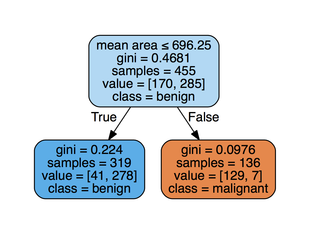
This caret API is so cool you can use it for lots of models. You’ll build random forests below. Before describing random forests, you’ll need to know a bit about decision tree classifiers. Decision trees allow you to classify data points (also known as “target variables”, for example, benign or malignant tumor) based on feature variables (such as geometric measurements of tumors). See here for an example. The depth of the tree is known as a hyperparameter, which means a parameter you need to decide before you fit the model to the data. You can read more about decision trees here. A random forest is a collection of decision trees that fits different decision trees with different subsets of the data and gets them to vote on the label. This provides intuition behind random forests and you can find more technical details here.
Before you build your first random forest, there’s a pretty cool alternative to train test split called k-fold cross validation that we’ll look into.
Cross Validation
To choose your random forest hyperparameter max_depth, for example, you’ll use a variation on test train split called cross validation.
We begin by splitting the dataset into 5 groups or folds (see here, for example). Then we hold out the first fold as a test set, fit our model on the remaining four folds, predict on the test set and compute the metric of interest. Next we hold out the second fold as our test set, fit on the remaining data, predict on the test set and compute the metric of interest. Then similarly with the third, fourth and fifth.
As a result we get five values of accuracy, from which we can compute statistics of interest, such as the median and/or mean and 95% confidence intervals.
We do this for each value of each hyperparameter that we’re tuning and choose the set of hyperparameters that performs the best. This is called grid search if we specify the hyperparameter values we wish to try, and called random search if we search randomly through the hyperparameter space (see more here).
You’ll first build a random forest with a grid containing 1 hyperparameter to get a feel for it.
# Create model with default paramters
control <- trainControl(method="repeatedcv", number=10, repeats=3)
metric <- "Accuracy"
mtry <- sqrt(ncol(df))
tunegrid <- expand.grid(.mtry=mtry)
rf_default <- train(X2~., data=df, method="rf", metric=metric, tuneGrid=tunegrid, trControl=control)
print(rf_default)
Random Forest

569 samples
 31 predictor
  2 classes: 'B', 'M'

No pre-processing
Resampling: Cross-Validated (10 fold, repeated 3 times)
Summary of sample sizes: 511, 513, 512, 513, 513, 512, ...
Resampling results:

  Accuracy   Kappa
  0.9625076  0.9193644

Tuning parameter 'mtry' was held constant at a value of 5.656854
Now try your hand at a random search:
# Random Search
control <- trainControl(method="repeatedcv", number=5, repeats=3, search="random")
mtry <- sqrt(ncol(df))
rf_random <- train(X2~., data=df, method="rf", metric=metric, tuneLength=15, trControl=control)
print(rf_random)
Random Forest

569 samples
 31 predictor
  2 classes: 'B', 'M'

No pre-processing
Resampling: Cross-Validated (5 fold, repeated 3 times)
Summary of sample sizes: 455, 456, 455, 456, 454, 456, ...
Resampling results across tuning parameters:

  mtry  Accuracy   Kappa
   2    0.9578156  0.9092135
   6    0.9619042  0.9180916
  12    0.9613194  0.9168014
  15    0.9607345  0.9154082
  16    0.9619092  0.9180466
  18    0.9625044  0.9193323
  19    0.9607242  0.9155330
  21    0.9624992  0.9192701
  23    0.9577897  0.9091203
  24    0.9601598  0.9143988
  25    0.9589697  0.9117203
  28    0.9601341  0.9142834
  30    0.9589696  0.9118957

Accuracy was used to select the optimal model using the largest value.
The final value used for the model was mtry = 18.
And plot the results:
plot(rf_random)

Key Points
The target variable is the variable of interest, while the rest of the variables are known as features or predictor variables.
Separate your data set into training and test sets to avoid overfitting.
Logistic regression and random forests can be used to predict categorical variables.